Experimenting with GGML: A Beginner's Guide to Efficient Inference

Feb 25, 2024

Note: This blog post is part of my ongoing work on experiments with model training, deployment and monitoring repository bitbeast.

Source Code: GitHub

Introduction

The domain of machine learning model inference is rapidly evolving, driven by the need for faster, more efficient models that can operate on resource-constrained devices. Techniques like quantization, knowledge distillation, and the use of specialized hardware like GPUs and TPUs make it possible for complex models to be available for real-world applications in different types of devices. Large Language Models (LLMs) upped the ante for inference, demanding faster processing for their complex nature and real-time applications. Efficient vector calculations are the key to unlocking potential, not just for LLMs but all complex models, and researchers are making strides with optimized algorithms and specialized hardware. One recent advancement that contributes to such effort is GGML.

GGML for LLMs and Everyone

GGML is a C library that enables efficient inference. It empowers LLMs to run on common hardware, including CPUs and Apple Silicon, using techniques like quantization for speed and efficiency. It boasts features like automatic differentiation, built-in optimization algorithms, and WebAssembly support, making it a versatile tool for developers working with LLMs at the edge.

Here are some noteworthy examples from the community:

Llama2.c - Inference Llama 2 in one file of pure C
whisper.cpp - Port of OpenAI’s Whisper model in C/C++
stable-diffusion.cpp - Stable Diffusion in pure C/C++

While initial exploration of GGML can be challenging due to limited documentation, I undertook on a hands-on learning journey by training a tiny neural network, converting it and running inference in C/C++. Let’s delve into the insights I gained while experimenting with GGML for the very first time!

Experimenting With Tiny Model

Let’s build a very simple neural network for learning a 2-input truth table:

class Model(nn.Module):
    def __init__(self):
        super(Model, self).__init__()
        self.fc1 = nn.Linear(2, 16)  # First hidden layer with 16 neurons
        self.relu = nn.ReLU()  # Activation function for hidden layer
        self.fc2 = nn.Linear(16, 1)  # Output layer with 1 neuron
        self.sigmoid = nn.Sigmoid()  # Activation function for output layer

    def forward(self, x):
        x = self.fc1(x)
        x = self.relu(x)
        x = self.fc2(x)
        x = self.sigmoid(x)
        return x

We will train this network on a truth table of our choice: XOR, OR or AND (or basically whatever you like!). For example, XOR will have inputs: [[0, 0], [0, 1], [1, 0], [1, 1]] and [[0], [1], [1], [0]].

Using PyTorch’s inbuilt functionality we can save the weights like:

torch.save(model.state_dict(), 'weights.pth')

At this stage, you can refer to model.py for the model training source code.
This is a great starting point, especially if you’re already familiar with PyTorch! As we progress, there might be some complexities.

Understanding GGML

GGML Binary File Format

In order for running inference using GGML we need to load model and its weights. Usually it depends on framework and its specification. GGML uses a binary file format for efficient storage of model weights. The format is agnostic of the machine learning framework, which means your model can be any of Keras, Tensorflow, PyTorch, MXNet, JAX, etc. Lets try to understand how we packed it for this tiny neural network written in PyTorch:

output_stream = open("assets/model.bin", "wb")
for name in model_state_dict.keys():
    data = model_state_dict[name].squeeze().numpy()
    # number of dimensions
    num_dims = len(data.shape)
    output_stream.write(struct.pack("i", num_dims))
    # dimension length and data
    data = data.astype(np.float32)
    for i in range(num_dims):
        output_stream.write(struct.pack("i", data.shape[num_dims - 1 - i]))
    data.tofile(output_stream)

output_stream.close()

This Python code acts like a translator for machine learning models by converting it into a more universal format. It does this by carefully breaking down the model’s components, noting their size and function, and then storing them efficiently in a single file. While the technical details involve packing data and dimensions, the core idea is streamlining the model for a wider use and potential adaptation.

There are specifics of GGUF, the new format in the GGML repository. While a full explanation of the new format’s principles is beyond our scope, you can find detailed resources online for those interested in diving deeper.

A simple explanation of the conversion code for our neural network would be:

Write the number of dimensions (num_dims) as a 4-byte integer ("i" format in struct.pack).
For each dimension:
- Write the length of the dimension as a 4-byte integer ("i" format in struct.pack).
Write the tensor data as a sequence of 4-byte float values (np.float32) using data.tofile(output_stream).

So it would pack the binary file:

fc1.weight:
- Number of dimensions (num_dims): 2 (since it's a 2D array)
- Dimensions: 16, 2 (shape of the weight matrix)
- Tensor data: -0.5434845, -0.8491827, ..., 0.3621676 (values of the weight matrix)

fc1.bias:
- Number of dimensions (num_dims): 1 (since it's a 1D array)
- Dimensions: 16 (length of the bias vector)
- Tensor data: 0.84919107, 0.76988536, ..., -0.71772271 (values of the bias vector)

fc2.weight:
- Number of dimensions (num_dims): 1 (since it's a 1D array)
- Dimensions: 16 (length of the weight vector)
- Tensor data: -1.0962133, -1.1020831, ..., -0.00229721 (values of the weight vector)

fc2.bias:
- Number of dimensions (num_dims): 0 (since it's a scalar)
- Tensor data: -0.32495027780532837 (single value of the bias scalar)

So far so good, we have successfully converted our trained PyTorch model into a GGML file format, which now can be read using C/C++ code. So let’s dig into that!

C/C++ Inference Code

For running inference using GGML, you will need to start by defining your neural network. Something like:

struct ptmodel_hparams {
    int32_t n_input   = 2;
    int32_t n_hidden  = 16;
    int32_t n_output = 1;
};

struct ptmodel {
    ptmodel_hparams hparams;
    struct ggml_tensor * fc1_weight;
    struct ggml_tensor * fc1_bias;
    struct ggml_tensor * fc2_weight;
    struct ggml_tensor * fc2_bias;
    struct ggml_context * ctx;
};

The idea is to initialize this network using the contents of a GGML format binary file. You can see the load function in main.cpp that performs this task.

Loading the weights

For running the inference, a model context is initialized using the ggml_init function, which essentially sets up a memory pool based on the total bytes required to define the model. You perform a binary read from the file created as mentioned before and assign values to model structure members using ggml_new_tensor_2d and ggml_new_tensor_1d functions (refer to the GGML source code for more details). These functions take the dimensions and data type (e.g., FP32, FP16) as arguments.

Running the vector calculations

Now, the actual magic happens in the predict function in main.cpp:

struct ggml_context * ctx0 = ggml_init(params);
struct ggml_cgraph * gf = ggml_new_graph(ctx0);

struct ggml_tensor * input = ggml_new_tensor_1d(ctx0, GGML_TYPE_F32, hparams.n_input);
memcpy(input->data, table_input.data(), ggml_nbytes(input));
ggml_set_name(input, "input");

ggml_tensor * fc1 = ggml_add(ctx0, ggml_mul_mat(ctx0, model.fc1_weight, input),                model.fc1_bias);
ggml_tensor * fc2 = ggml_add(ctx0, ggml_mul_mat(ctx0, model.fc2_weight, ggml_relu(ctx0, fc1)), model.fc2_bias);

ggml_tensor * probs = ggml_hardsigmoid(ctx0, fc2);
ggml_set_name(probs, "probs");

ggml_build_forward_expand(gf, probs);
ggml_graph_compute_with_ctx(ctx0, gf, 1);

We begin by initializing a GGML context, which manages memory and operations for tensors and graphs. Additionally, we create a new computational graph within the context to represent the model’s computations.

Similar to the load function, we take the input and convert it into a ggml_tensor_1d using ggml_new_tensor_1d.

We perform a basic matrix multiplication between the input and the first layer using ggml_mul_mat, followed by adding its bias. Additionally, we also use the ggml_relu and ggml_hardsigmoid functions, which aim to mimic the functionalities of torch.nn.ReLU and torch.nn.Sigmoid, respectively. Invoke the forward pass execution on the graph and context using ggml_build_forward_expand.

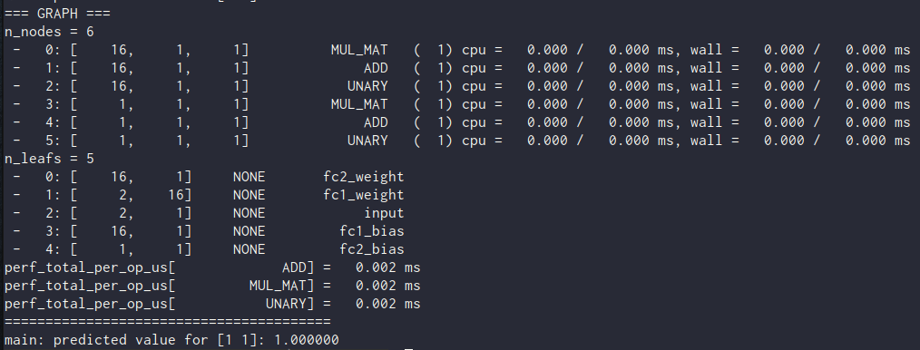GGML Example Graph <code>ggml_graph_print</code>

GGML Example Graph, Output of ggml_graph_print

The graph visualizes the sequence of operations performed by the model, including data movement, mathematical computations, and activation functions. By following the connections between nodes, you can understand how the input data is transformed through different layers to produce the final output. It also provides the execution times or resource usage associated with different nodes can help pinpoint potential bottlenecks or inefficiencies in the model’s computation.

Boom! You’ve successfully built, saved, and run a model using GGML. It is just the tip of the iceberg, though. We’ve barely scratched the surface of what’s possible. Dive deep by exploring different examples mentioned in GGML README. There is some scope to do some Quantization but I will save that for later!

If you liked the idea of pytorch.cpp, go check it out on GitHub. If you have an idea or a suggestion for improvement, feel free to contribute via Issues/Pull Requests!